Yes, high yield bonds’ true duration is… negative

When we first published this white paper in early 2021, we noted that all the analysis happened after inflation was subdued in the 1980s. In the 13 cycles where Treasury rates increased, high yield credit spreads also compressed and high yield bonds exhibited negative empirical durations and, thus, positive returns.

However, we also noted that, should higher rates be accompanied by higher inflation, we would likely see falling high yield prices. That is exactly what happened in 2022. High yield bond prices, traditionally poorly correlated with Treasuries, suddenly have become much more highly correlated. If stagflation ensues, we would expect high yield bonds to behave more like investment grade bonds, with returns driven in large part by Treasury rates, not corporate performance. But if we see core inflation materially recede from current levels while real economic growth remains positive, we would expect high yield to more closely mirror the returns of equities, an asset class to which it is closely correlated, as both high yield and equities would respond to the health of the economy.

Duration is a common tool of fixed income analysis, used to calculate how much a bond portfolio will gain or lose value in response to a change in interest rates. It works quite well for the various types of investment grade debt, and adaptations such as effective duration and convexity have been developed to formally incorporate the effect of embedded call options on those price movements. However, we contend that duration is almost meaningless as a tool for predicting the behavior of high yield bond prices. 

In fact, it consistently fails to predict even the direction of price changes, and in a way which varies systematically with bond quality. This paper shows why empirical durations of high yield bonds, proven by actual (not predicted) bond prices, are actually consistently negative.

The first three months of 2021 have brought highly negative returns for Treasuries and investment grade corporate bonds, while high yield bonds have eked out slightly positive returns of 0.65% through March 29 and leveraged loans have returned 2.01% (for an annualized and compounded 8.29%.) Observers of the bond markets should be experiencing a feeling of déjà vu. Figure 1 reveals that not only are these relative returns, and their signs, not unusual, but they have occurred in every single period of rising rates since at least 1993.

FIGURE 1: FIXED INCOME IN RISING RATE ENVIRONMENTS¹: HIGH YIELD VS IG

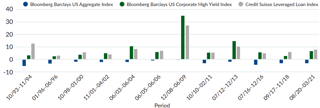
​Source: Bloomberg & Credit Suisse.

We are always a bit befuddled when we are asked about the duration of our portfolio and how we “manage” duration. We wonder which duration is of concern…the conventional measurement, or the way our portfolio empirically responds to changes in Treasury rates? All the conventional measurements of duration—Macaulay duration, modified duration, effective duration, option-adjusted duration, and the like—are purely mathematical constructs which measure the theoretical price response of a bond when rates rise or fall. Though some of these adjust for the embedded call options in most corporate bonds, they all ignore the most important feature of high yield bonds—the fact that default risk introduces large (and more important, variable) differences between promised cash flows and the expected cash flows that actually determine values of bonds.

Recently, respected researchers at Bank of America/Merrill Lynch (BAML) published a short note in which they systematically calculated the empirical durations of corporates of different ratings over a ten year period, using weekly returns and the five year Treasury rate as the reference point. Their extremely important results, published with permission, are presented in Figure 2. In brief: investment grade bonds do fall in price when rates rise. But high yield bond prices go up.2 

FIGURE 2: EMPIRICAL DURATIONS BY RATING

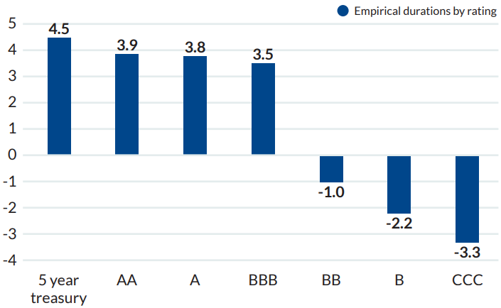
Source: Oleg Melentyev and Eric Yu, Bank of America/Merrill Lynch High Yield Strategy, September 4, 2020.

Note that investment grade bonds of all ratings do have positive empirical durations, but high yield bonds actually have negative durations, which become increasingly negative as we descend from BB to CCC. High yield bonds are not immune to the mathematical fact that a more heavily discounted cash flow will lose value, but they uniquely have expected (not promised) cash flows which themselves change when rates are higher. During the low-inflation era since the 1980s, rising rates have generally occurred at a time when the economy is improving, and a stronger economy means that expectations of default rates are falling. Cash flow is more highly discounted, but there is more expected bond cash flow to begin with when the economy is booming, and this latter effect is stronger than the purely mathematical effect of more discounting. The net effect is that bond prices rise along with rates. Viewed in this way, it is not a surprise that CCC prices rise more than B prices, which in turn rise more than BB prices: CCC bonds begin with a higher expected default rate, so a downward revision to those expected defaults is logically a more powerful influence on value than it is for a safer B or BB rated bond.

This is another way in which the “hybrid” nature of a high yield bond becomes evident. Correlation analysis of long term returns shows that all classes of high grade debt—Treasuries, corporates, mortgages, and the like—exhibit correlations with each other exceeding 80%. But the asset class to which high yield debt is most correlated (after its sister asset, leveraged loans) is not a fixed income category at all—it is equities, because both are responding to the health of the economy. High yield is 72-78% correlated to various equity indices, but only 21% correlated to the leading investment grade index, the Barclays (formerly Lehman) Aggregate.3

The appendix to this short paper illustrates in detail how the rate effect and the change in expected cash flows work to produce a negative empirical duration.

We like this analysis of the effect of interest rates on bond prices because it is demonstrable using the logic of present value of expected cash flows. Many market practitioners express the same effect in a different way, speaking in terms of credit spreads: “When rates rise, credit spreads compress, and so high yield does not get hurt as badly as investment grade debt.”  We prefer to express the change in terms of bond prices, not spreads, because the entire concept of duration as a tool is directed at making a statement about prices: “If rates rise 100bp, your portfolio will fall by 3%.”  And focusing on prices, and negative empirical duration, makes clear that  not only do spreads compress, but they compress by enough to make the bond price actually rise, not just fall by less than an investment grade bond would.

From the point of view of an allocator constructing a portfolio, we believe the negative empirical duration is the correct way to think. This will strike many as a novel idea, and it certainly has the feel of “fuzzy logic” when juxtaposed with the precision conventional duration brings to investment grade analysis. A CIO forced to think of the big picture probably uses software that makes conclusions such as “the mathematical duration of your high grade portfolio is 6 years, the mortgage portfolio is 5, and the high yield portfolio is 3 years, for a weighted average of 4.5 years.” But remember, the whole reason to care about duration is not the number itself, but rather its usefulness as a predictor of the actual value of the portfolio when rates move. Use of empirical duration would take advantage of the fact, being seen again today, that a high yield portfolio is actually a natural economic hedge to a high grade universe whose duration has been significantly lengthening in recent years. Ten years ago, the duration of the Barclays Aggregate was about 5 years. Today, it is 6.4 years. 

Will the robust inverse relationship between interest rates and high yield bond prices hold up in the future? This turns on why rates might rise. As noted earlier, all of the analysis in this paper happened after inflation was subdued in the 1980s, and inflation has remained low ever since. Thus, interest rates have been mostly “real” and not heavily impacted by inflationary expectations. But there are reasons to think this may be changing. The monetary base has grown very rapidly lately, the Fed’s balance sheet has grown massively for a decade through the various phases of “easing,” and the current administration has embraced the novel ideas of “modern monetary theory.” Monetary velocity has dropped more or less continuously since 1997, and precipitously so during the lockdowns of 2020, and this has kept prices from breaking out. Although this is not the place (nor am I the author) to opine on monetary economics, there is certainly the potential for higher inflation expectations to become a co-driver of Treasury rates in a way that we have not seen in decades. 

We would expect that empirical durations of high yield bonds will be less negative in an inflationary environment with underlying strong real growth, as we expect in 2021. But if stagflation ensues, rising rates can become decoupled from strong growth, and at that point we would expect high yield bonds to behave more like investment grade bonds. Absent high growth, pure inflation (decoupled from real growth) hurts all fixed coupon assets. Nominal revenues, profits, and asset values would rise, bond prices would fall, and inflation would drive a wealth transfer from bond holders to equity holders.

Turning to the behavior of leveraged loans when rates rise, a re-examination of Figure 1 shows that in some periods of rising rates, loans outperform high yield bonds, and vice versa. This makes sense too. Leveraged loan coupons reprice quickly when their short term “base rate” (usually LIBOR) changes, so the pure rate effect on a leveraged loan’s price is near zero. However, the contractual spread over LIBOR is unaffected by changes in the base rate, and if rates are rising because economic prospects are improving, then the contractual spread in an existing will become wider than newly priced loans of equal risk, so that loan’s price will appreciate.4

Appendix

HOW THE PURE RATE EFFECT AND THE CHANGE IN EXPECTED CASH FLOWS DETERMINE NEGATIVE DURATION

When we speak of a bond “trading at an 8% yield” we are speaking imprecisely in an important way. The promised coupon and principal payment at maturity can indeed represent a promised nominal yield of 8%, but every buyer of high yield bonds realizes that the yield is high precisely because it is only promised…there is a real risk that it will not be paid, and so the borrower must promise a nominal rate of return which is high enough to make the lender believe that the probability-weighted expected realized return will still be substantially higher than an otherwise comparable bond with little or no default risk. The long term net default loss rate (after accounting for recoveries) on B rated high yield bonds is 2.5%. A correct statement would be: “I am buying a bond at a promised yield of 8% but over many “trials” in the portfolio, I am expecting to realize 5.5% if I hold it to maturity.” 

Imagine such a non-callable bond purchased at issue with a maturity of five years and, for simplicity, annual coupons. The annual gross expected default rate is 4.2%, but if the bond defaults it will be converted to cash at a value of 40% of par…thus, the net default loss rate is the aforementioned 
4.2% *(1 - 40%) = 2.5%. 

The expected cash flow (expected coupon plus expected partial principal return in the event of default) in year 1 is (8 * 95.8%) + (40 *4.2%) = 9.34

The expected cash flow in year 2 is (8 * 95.8% * 95.8%) + (40* 4.2% * (1 - 4.2%)) = 8.95

And so on for years three, four, and five. The total expected cash flow from this bond over its life is 123.6 - materially below its promised total principal and interest of 140. That’s why it’s a high yield bond.

Now suppose that the economy strengthens and five-year Treasury rates rise by 100 basis points…not unlike what has happened in the last few months. Bond investors would be faced with re-estimating the default probability over the next five years under these new conditions. And it turns out that high yield default rates are highly variable. For B rated bonds, if we look at all five-year periods in the S&P default database, the lowest quintile 5-year default loss rate is 1.02%, the third quintile loss rate is 2.6%, and the highest quintile 5-year default loss rate is 4.3%. The investor, and the market, may believe that after rates have shifted up and the economic outlook has improved, the forward-looking default loss rate has shifted from the average value of 2.5% to, say, 1.30%, which would be at about the 25th percentile mark. That is to say, the economy has strengthened such that the revised default expectation is now better than 75% of all prior five-year periods instead of being average. (For context, that 1.30% expected loss rate would be about equal to the actual loss rate in the five year period after the last recession.) 

The total expected cash flow of the bond would move up significantly—to 131.3, an increase of 6.2% over what it was in the more economically neutral, lower-rate environment in which it was purchased. 

We can now tie together the two separate influences on empirical duration. The bond at purchase had a Macaulay duration of 4.3 years and a modified duration of 4.0 years. Thus, the pure rate effect on price from the 1% rate rise would be the conventionally calculated loss in value of 4%. However, there is 6.2% more in expected cash flow to discount. The net change in value is a positive 2.2%...and equal to the result from the negative 2.2 empirical duration of B rated bonds found by the BAML researchers. It can be seen that for BB rated issuers, the improvement in expected defaults would be lower than for the B rated bond, and thus the increase in cash flow would be lower, and so BB rated bonds would have a less negative empirical duration. For CCC rated bonds, the improvement in prospective default rates would be higher, the increase in expected cash flow correspondingly greater, and the empirical duration more strongly negative, just as the BAML research found.

It can also readily be seen why investment grade bonds have positive durations that are very close to the durations of Treasury bonds. Historical default loss rates on investment grade bonds are trivial—per Standard and Poor’s data since 1981, zero for AAA and AA debt, 3bp per year for A rated debt, and about 12bp per year for BBB rated debt. These loss rates are already so low that a strengthening economy cannot depress them much before they reach the boundary value of zero. Those bonds’ expected cash flows cannot increase, so they are fully exposed to the pure rate effect on value with no countervailing benefit from lower expected default rates. 

Some readers may be moved to protest that “no one really thinks in this very formal way.” That is, that money managers do not think about a precise mathematical linkage between changes in Treasury rates and expected default rates in the quantitative way I have described, with varying coefficients for bonds of different ratings. For some managers, that is true. But markets exist to aggregate a set of opinions, both those which are carefully arrived at and those which are purely reactive, and the prices which underlie the negative durations we have observed do have a pattern which is appealingly explained by the theory in this paper. Managers implicitly rely on this type of analysis every time they engage in algorithmic “correlation trading” which is based on empiricism rather than economic logic. It is not necessary that any market participant actually think in this way for a market consensus to evolve which acts as if every manager responded to changes in rates as we have described herein.

​

DOWNLOAD

FOR EDUCATIONAL, INSTITUTIONAL AND INFORMATIONAL PURPOSES ONLY. There can be no assurance that any performance or results based on examples of duration strategies discussed herein will be achieved and materially different results may occur. Please see the disclosures at the end for additional, important information.

Past performance is not indicative of future results.

1. Trough-to peak rates in the ten year Treasury, with a minimum move of 100bp.

2. Oleg Melentyev and Eric Yu, Bank of America/Merrill Lynch High Yield Strategy, September 4, 2020.

3. JPMorgan 2020 High Yield Annual Review, page 109, covering the 15 year period ending November 30, 2020.

4. The analysis for a loan is more complex than for a bond because three are more moving parts. Loans are callable at all times with a small or zero call premium, and when rates are very low the coupon may be driven not by LIBOR itself but rather a contractual “floor” value for the base rate. And loans, having generally lower default loss rates than bonds, will have a correspondingly smaller upward revision in expected cash flows for a given improvement in the macroeconomic picture.

Mesirow refers to Mesirow Financial Holdings, Inc. and its divisions, subsidiaries and affiliates. The Mesirow name and logo are registered service marks of Mesirow Financial Holdings, Inc. © 2021. All rights reserved. Mesirow High Yield (“MHY”) is a division of Mesirow Financial Investment Management, Inc., (“MFIM”) an SEC-registered investment advisor. This communication is for institutional use only and may contain privileged and/or confidential information. It is intended solely for the use of the addressee. If this information was received in error, you are strictly prohibited from disclosing, copying, distributing or using any of this information and are requested to contact the sender immediately and destroy the material in its entirety, whether electronic or hardcopy. Nothing contained herein constitutes an offer to sell or a solicitation of an offer to buy an interest in any Mesirow investment vehicle. The information contained herein has been obtained from sources believed to be reliable, but is not necessarily complete and its accuracy cannot be guaranteed. Any opinions expressed are subject to change without notice. It should not be assumed that any recommendations incorporated herein will be profitable or will equal past performance. Performance information that is provided gross of fees does not reflect the deduction of advisory fees. Client returns will be reduced by such fees and other expenses that may be incurred in the management of the account. Advisory fees are described in Part 2 of Form ADV of MFIM FI HY. Yields are subject to market fluctuations. Mesirow Financial Investment Management, Inc. and its affiliated companies and/or individuals may, from time to time, own, have long or short positions in, or options on, or act as a market maker in, any securities discussed herein and may also perform financial advisory or investment banking services for those companies. Mesirow does not provide legal or tax advice. Securities offered by Mesirow Financial, Inc. member FINRA, SIPC. Additional information is available upon request. It is not for use with the general public and may not be redistributed. There can be no assurance that any performance or results based on examples of duration strategies discussed herein will be achieved and materially different results may occur.